Writing Custom Layers with Flux - With a Unet #

Flux is a very versatile library. In particular, it doesn’t have a strict interpretation of “layers” as one would find in most libraries. In fact, in more recent research into implicit representation of models and data, we now have models with infinite layers. Instead, Flux focusses on transformations. Having said that, it is still useful to have some abstractions that keep things organised.

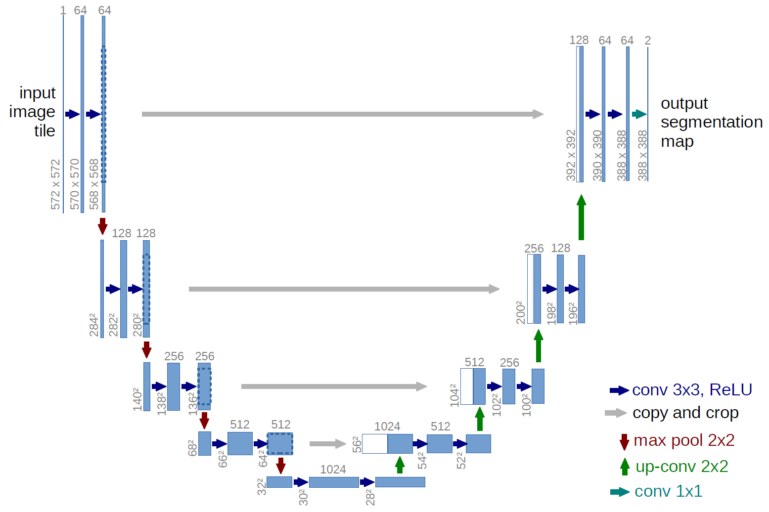
This post will focus on writing a UNet in Flux, and show how it can be used for deep learning. We will use it to write our own custom layers in the process. It is a fairly well aged network, and finds applications in medical imaging, but can be applied to a vast gamut of fields and perform image segmentation tasks in general. In that way, it is a part of natural progression from image classification to object detection and localisation to semantic segmentation and beyond. Here is a brief overview of the network in question.

Architecture #

UNet has been applied to a large number of problems like Autonomous Driving, since it is useful to detect lane markings, traffic signs and even free space for the cars to move into. It has also been applied to Geo-Sensing and Land Cover analysis for helping with various projects including city planning and traffic management. You might be interested in this blog that goes deeper into UNet itself.

No points for guessing how it got its name, though.

Further, since its a fully convolutional model, it can also be used by images of arbitrary sizes.

The reference implementation of the model in PyTorch can be found here.

Writing Layers #

Writing a layer in Flux is actually pretty straightforward, getting rid of most boilerplate code. Ii is fairly standard practice to define ones own structs to use in specialisation and method dispatch in Julia. We will use structs to define our layers.

Thinking of the components to define a layer, we need to figure out what kinds of parameters it can hold, and what happens when the layer is fed some input. For this post, we can assume the inputs are going to be regular arrays.

Basic Scaffolding for a Layer #

The general style guide to define the layer, would look so:

struct MyLayer
  a
  b
  c
end

function (a::MyLayer)(x::AbstractArray)
  # do something...
end

Simple Explanation #

Here, our layer would hold some parameters (and peripheral details; think padding for a convolutional layer) in its fields (a,b,c...). We then make this layer callable (known as a functor); this isn’t strictly necessary since we can define a normal function that takes a layer object explicitly, like usual, but doing this allows us to use layer in a much more natural looking manner:

MyLayer(input)

There is one additional operation that Flux expects, which is calling @functor MyLayer. It makes it such that all the parameters of our layer are visible to the AD, while backpropagating. This can be thought of in a way “registering” the layer to take advantage of the rest of the machinery.

Note: that if only certain fields are designed to be treated as parameters, leaving the rest of them untouched, it is possible to call

@functor MyLayer a, b

Beyond this, we will exploit one other possibility that this opens up. This is the ability to compose layers together, creating higher-order layers. Composing these layers together basically makes up the models, with their own forward pass implicitly defined.

Translating this Pattern to a UNet #

Let me demonstrate that with an example. The UNet has a bunch of structures within itself that is symmetric around the smaller convolutional structure. We’ll call them UNetUpBlock, as it does upsampling.

struct UNetUpBlock
  upsample
end

@functor UNetUpBlock

function (u::UNetUpBlock)(x, bridge)
  x = u.upsample(x)
  return cat(x, bridge, dims = 3)
end

So far so good. This looks very similar to the template we had prepared from earlier. Now, let’s add some convenience methods to UNetUpBlock so its simpler to construct.

UNetUpBlock(in_chs::Int, out_chs::Int; kernel = (3, 3), p = 0.5f0) =
    UNetUpBlock(Chain(x -> leakyrelu.(x,0.2f0),
                ConvTranspose((2, 2), in_chs => out_chs,
                        stride = (2, 2); init = _random_normal),
                BatchNormWrap(out_chs)...,
                Dropout(p)))

I’ve left the definition of some functions (such as BatchNormWrap and _random_normal) out of this tutorial for clarity, but all the functions can be found in UNet.jl.

Notice, it isn’t strictly necessary to write a new layer in this case, since we really just need the forward pass to run on the upsample field, which in itself is just a tiny model! Here, defining this layer only really is helping us avoid rewriting the forward pass with the concatenation multiple times. If we hadn’t needed this, it is possible to just define a simple function that captures the cat function with the x and bridge variables. Next, we need to downsample. This would look like a mirror of the UNetUpBlock, the ConvDown layer:

ConvDown(in_chs,out_chs,kernel = (4,4)) =
	Chain(Conv(kernel,in_chs=>out_chs,
		   pad=(1,1),
		   stride=(2,2);
		   init=_random_normal),

	      BatchNormWrap(out_chs)...,
	      x -> leakyrelu.(x, 0.2f0))

Composing Layers Together #

We can now use these layers to simplify our construction of the actual UNet, which can itself be described as just another layer.

struct UNet
  conv_down_blocks
  conv_blocks
  up_blocks
end

@functor UNet

function UNet()
  conv_down_blocks = Chain(ConvDown(64,64),
                      ConvDown(128,128),
                      ConvDown(256,256),
                      ConvDown(512,512))

  conv_blocks = Chain(UNetConvBlock(1, 3),
                 UNetConvBlock(3, 64),
                 UNetConvBlock(64, 128),
                 UNetConvBlock(128, 256),
                 UNetConvBlock(256, 512),
                 UNetConvBlock(512, 1024),
                 UNetConvBlock(1024, 1024))

  up_blocks = Chain(UNetUpBlock(1024, 512),
                UNetUpBlock(1024, 256),
                UNetUpBlock(512, 128),
                UNetUpBlock(256, 64,p = 0.0f0),
                Chain(x->leakyrelu.(x,0.2f0),
                Conv((1, 1), 128=>1;init=_random_normal)))
  
  UNet(conv_down_blocks, conv_blocks, up_blocks)
end

The actual definition of the model is quite a bit clearer and makes it very obvious how the model is layed out. The left side of the model can be mapped to the conv_down_blocks and the upsampling ones to the up_blocks. Neat.

Putting All the Pieces Together #

Now to define the forward pass, we just need to remember that we want to first downsample the incoming image, apply the conv blocks, and finally upsample it back up to the size of the image. Remember that we modeled the whole thing as a layer? Well we can just define what we spoke about here as the forward pass. Following the paper, it would look a little like so:

function (u::UNet)(x)
  outputs = Vector(undef, 5)
  outputs[1] = u.conv_blocks[1:2](x)

  for i in 2:5
    pool_x = u.conv_down_blocks[i - 1](outputs[i - 1])
    outputs[i] = u.conv_blocks[i+1](pool_x)
  end

  up_x = u.conv_blocks[7](outputs[end])

  for i in 1:4
    up_x = u.up_blocks[i](up_x, outputs[end - i])
  end

  tanh.(u.up_blocks[end](up_x))
end

Since Flux can differentiate arbitrary code, we can take some liberties to define the layers and their forward passes like we did, eliminating any boilerplate, or specialised “blessed” functions to allow us to express the problem naturally. This way of defining layers is just one way to express them. As eluded to before, any function/ operation/ transformation is considered a layer in itself, with most having their gradients calculated on the fly.

Closing Thoughts #

The expressiveness the framework allows is one of those subtle differences from how most libraries are laid out. It also means we can just as easily start using other packages in our models as well. No need to have specially designed “differentiable” versions of tools, since in Julia, everything is differenitable by default. Well, almost everything 😉

Cheers